Filtering Data
Learn how to filter lists and tables to show only the records you need. Use checkbox filters, search, text/number/date filters, and clear filters confidently.
By the end of this lesson you can
- Apply and clear filters on one or more columns
- Use text, number, and date filters for specific criteria
- Explain what filtering hides and what it does not remove
- Recognize when filtered rows are affecting your totals
Video
Watch the lesson video, then complete the reading and challenge.
Lesson Notes
Read through the key concepts before you try the challenge.
Filtered rows are hidden, not gone
You report on medical supply spending at Lakeside Medical Associates.
You filter the sheet to Medical Supplies and read the total at the bottom: $18,400. That figure is the total of every row in the sheet, including the office and cleaning supplies currently hidden. You report it as the medical supply spend, and it is wrong by about two-thirds.
Your task: Understand that filtering changes what you see, not what formulas calculate.
Filtering hides rows that do not match. The data is entirely intact and returns when the filter is cleared — which is what makes it safe. But SUM and AVERAGE include hidden rows, because they operate on the range, not on what happens to be visible.
=SUBTOTAL(109, E2:E900) is the fix: it sums only visible rows and updates as the filter changes. The 109 specifies sum-ignoring-hidden-rows. There is a parallel code for each function — 101 for average, 103 for count. Converting the range to an Excel Table gives you a Total Row that uses SUBTOTAL automatically.
Why Filters Matter
When a worksheet has a lot of rows, it’s hard (and honestly pointless) to scroll forever hunting for what you need. Filters let you temporarily hide rows that don’t match your criteria—without deleting anything.
Filters are perfect for finding items by category, narrowing to specific dates, or showing only records that meet a numeric requirement (like loan amounts over $100).
Before You Filter: Make Sure You Have Headers
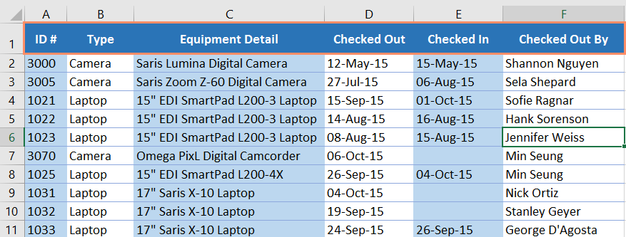
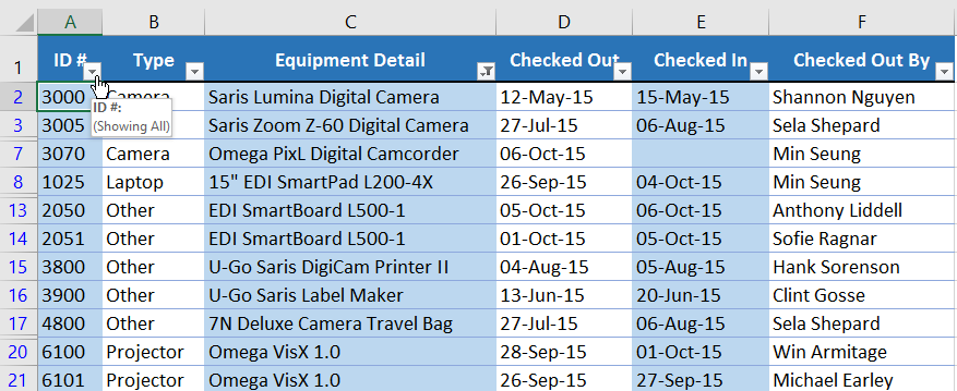
Filtering works best when your data has a clear header row (column names like ID#, Type, Item Description, etc.). Excel uses these headers to label each filter dropdown.
Turn Filters On
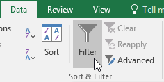
To enable filtering, go to the Data tab and click the Filter button. Excel adds a dropdown arrow to each header cell.
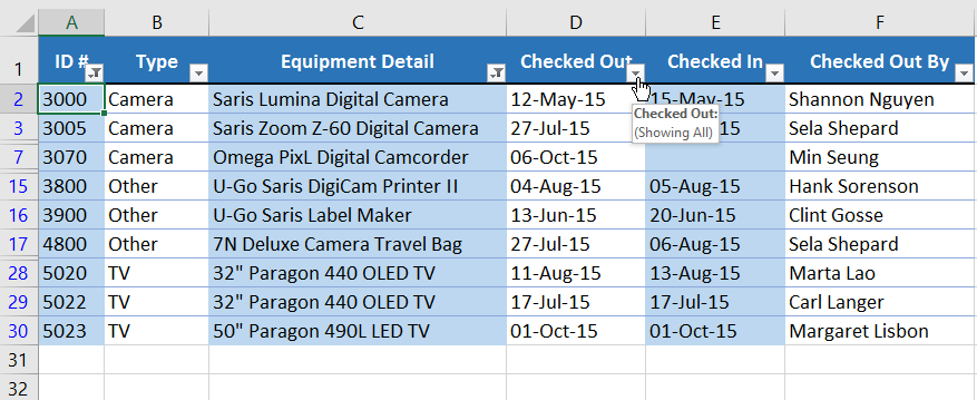
Once filters are on, every column header gets a dropdown arrow you can click to filter that column.
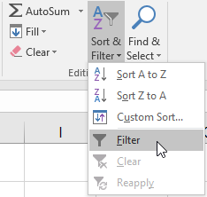
You can also access Filter from the Home tab under Sort & Filter (different path, same tool).
Basic Filtering with Checkboxes
The simplest filter is the checkbox list. You open the filter dropdown, uncheck everything, then check only what you want to see.
Example: Filter the Type column to show only Laptop and Projector.
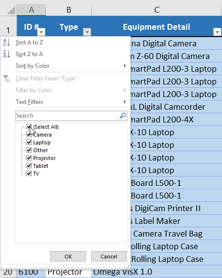
First, uncheck Select All so you can start from a clean slate.
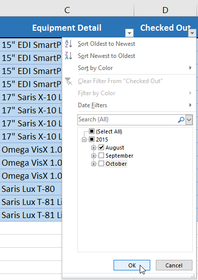
Then check only the values you want and click OK. Excel hides everything else.
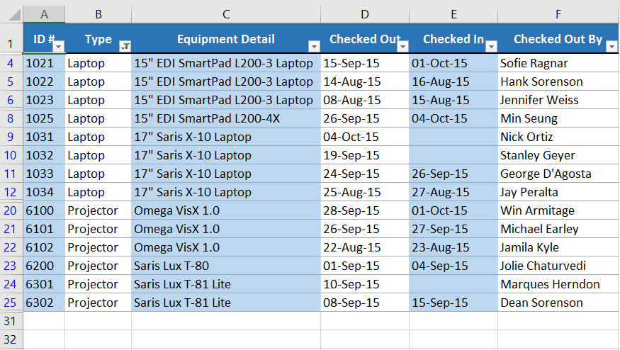
Applying Multiple Filters (Filters Stack)
Filters are cumulative—meaning each new filter further narrows your results. This is how you go from “a lot of rows” to “exactly what I need.”
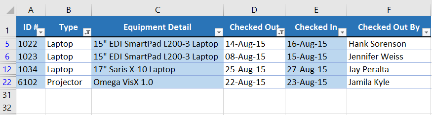
Example: If you already filtered Type to Laptop + Projector, you can ALSO filter Checked Out to show only items checked out in August.
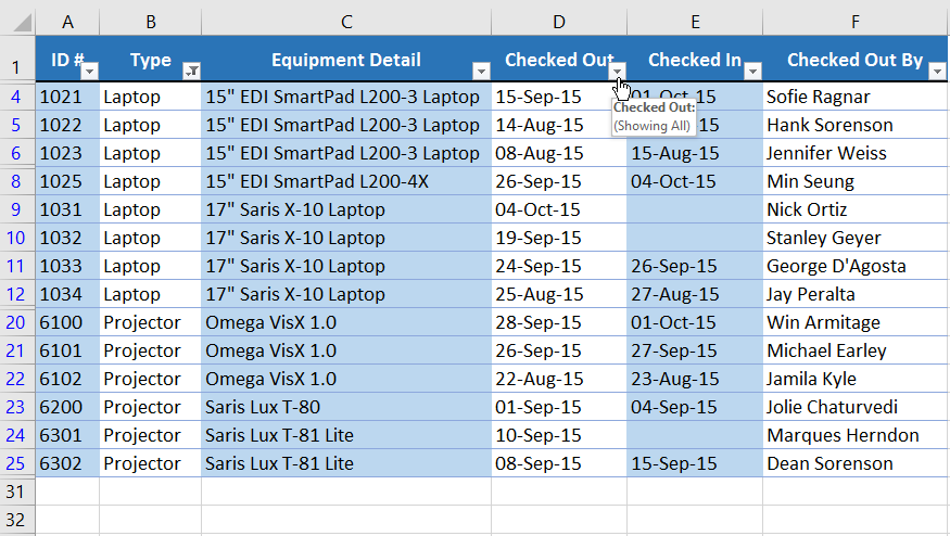
After applying that second filter, you’ll see a smaller subset that matches BOTH criteria.
Clearing a Filter (Without Turning Filters Off)
When you’re done with a filter, don’t panic-scroll. Just clear it.
Open the dropdown for the filtered column and choose Clear Filter From [Column Name]. That restores the hidden rows for that column’s filter.
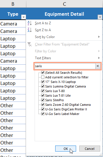
If you want to remove ALL filters from the sheet at once, click Filter again on the Data tab to toggle filtering off.
Filtering with Search
Search is the fastest way to filter when you’re looking for one brand, keyword, or repeated term.
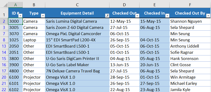
Open the filter dropdown for the column you want (like Equipment Detail), then type into the search box. Excel narrows the checkbox list automatically as you type.
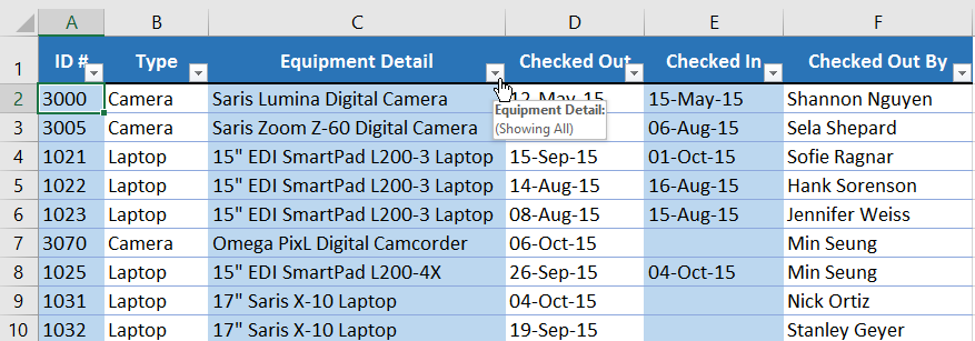
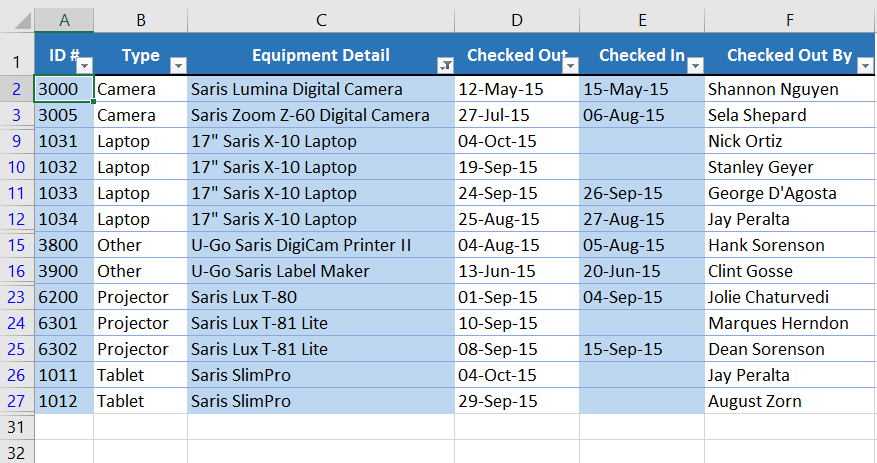
Example: Type saris to show only Saris items.
Advanced Text Filters (Contains / Does Not Contain)
When checkboxes and search aren’t specific enough, use Text Filters. These let you filter based on rules like Begins With, Ends With, Contains, or Does Not Contain.
Example: Exclude items that contain the word laptop.
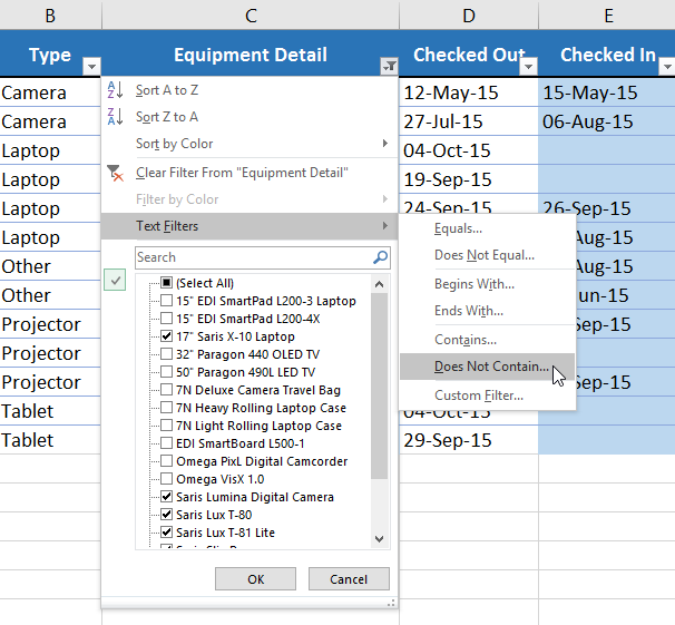
This opens a Custom AutoFilter box where you type the word or phrase and confirm.
Advanced Number Filters (Greater Than / Between)
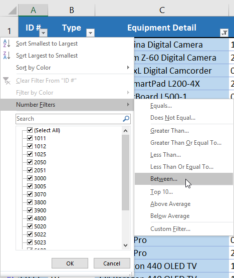
Number Filters are used for columns with numeric values like ID numbers, quantities, prices, or loan amounts.
You can filter values greater than, less than, between two numbers, top 10, above average, and more.
Example: Show only records with ID numbers between 3000 and 6000.
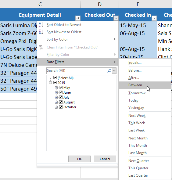
Advanced Date Filters (This Month / Between Dates)
Date filters are built for time-based data. You can filter by year, month, or use built-in ranges like Last Week, Next Month, or Between two dates.
Example: Filter Checked Out to show only items checked out between two specific dates.
Knowledge Check
What does applying a filter to a column do?
Practice File
Download this file and follow along with the lesson.
Challenge
Apply what you've learned in this lesson.
Download and open the practice workbook.
- Click the Challenge tab in the bottom-left of the workbook.
- Apply a filter to show only Electronics and Instruments.
- Use the Search feature to filter item descriptions that contain the word Sansei (you should see 6 entries).
- Clear the Item Description filter.
- Using a number filter, show loan amounts greater than or equal to $100.
- Filter to show only items that have deadlines in 2016.
- When you're finished, your workbook should look like the example below.

Finished this lesson?
Progress is saved in this browser only. It is not a grade — official progress lives in Brightspace.