Relative & Absolute Cell References
Learn how relative, absolute, and mixed references behave when formulas are copied, and how to reference cells across worksheets.
By the end of this lesson you can
- Explain how relative references shift when a formula is copied
- Use absolute references to anchor a formula to a fixed cell
- Use mixed references to lock only a row or only a column
- Cycle reference types with F4 while editing
Video
Watch the lesson video, then complete the reading and challenge.
Lesson Notes
Read through the key concepts before you try the challenge.
The dollar sign means 'do not move this'
You apply a tax rate across the supply sheet at Lakeside Medical Associates.
The rate is in F1. You write =E2*F1 in the first row and fill down. Row 3 becomes =E3*F2, row 4 becomes =E4*F3 — the reference slid down with the formula, off the rate and into empty cells. Every row below the first is now wrong, and most show a plausible-looking zero.
Your task: Control which parts of a reference move when a formula is copied.
A relative reference like F1 is really an instruction about position: 'the cell one column right and one row up from me.' Copy the formula down and that instruction is re-evaluated from the new location, which is why it slides. This is exactly what you want for =C2*D2, and exactly what you do not want for a rate cell.
A dollar sign freezes the part it precedes. $F$1 is fully absolute and never moves. F$1 locks the row but lets the column shift. $F1 locks the column but lets the row shift. These mixed forms are what let a single formula fill across a whole grid — a rate table where one axis is fixed by row and the other by column.
| Written | Called | When copied |
|---|---|---|
| F1 | Relative | Both column and row shift |
| $F$1 | Absolute | Never changes |
| F$1 | Mixed — row locked | Column shifts, row stays at 1 |
| $F1 | Mixed — column locked | Row shifts, column stays at F |
Understanding Relative References
Relative references are Excel’s default behavior. When a formula is copied, the row and column references adjust automatically.
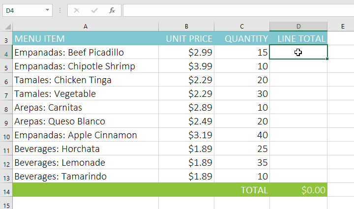
Click cell D4 first, then type an equals sign (=) to begin entering your formula.
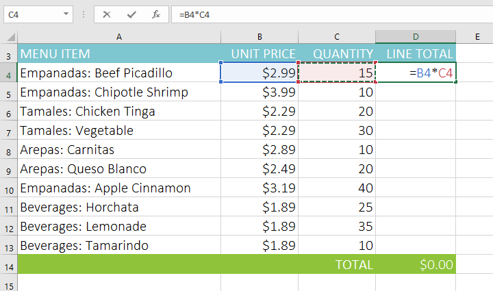
Enter the formula =B4*C4 to multiply Unit Price by Quantity.
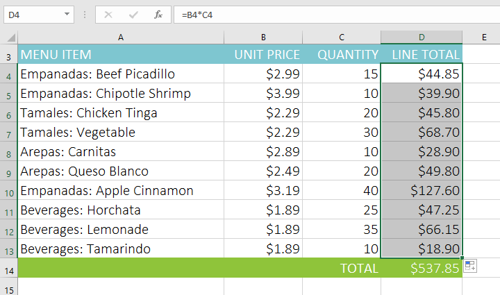
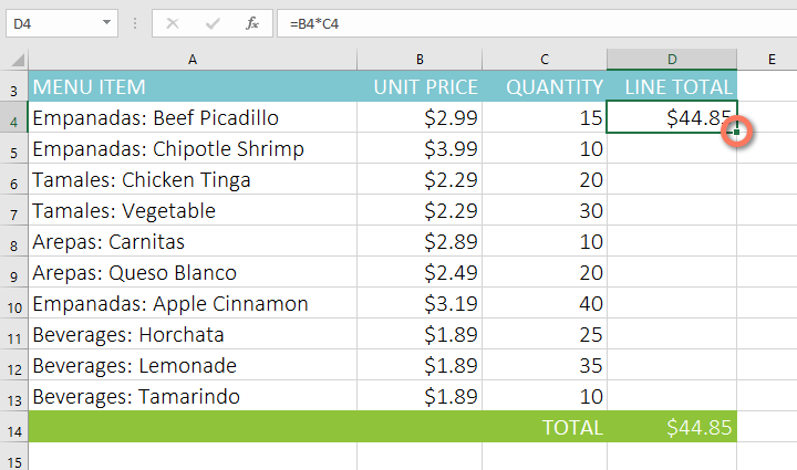
Use the fill handle to copy the formula downward.
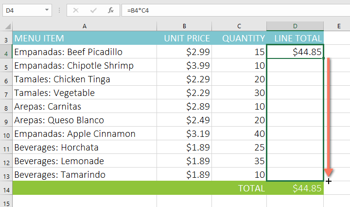
Notice how each row now references the corresponding unit price and quantity automatically.
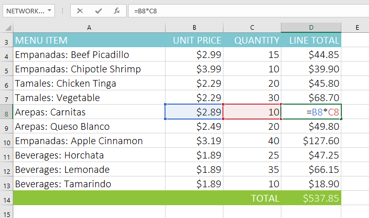
Because the references were relative, Excel adjusted the row numbers automatically as the formula was copied.
Locking a Cell with Absolute References
If a formula uses a value that should not change — such as a tax rate — we must lock the reference.
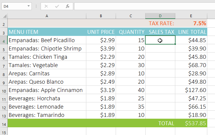
Without locking the tax rate in E2, copying the formula causes incorrect results.
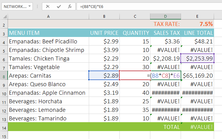
Because the reference was not locked, Excel shifted the tax rate cell as the formula was copied.
If you ever see your tax rate changing as you copy a formula, it usually means the reference was not locked.
Add dollar signs to lock the reference. $E$2 locks both the column and row. You can also click the cell reference and press F4 to insert the dollar signs automatically.
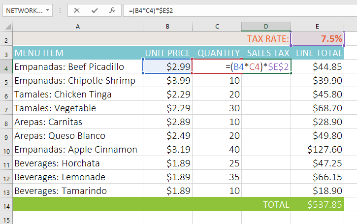
Now copy the formula down using the fill handle.
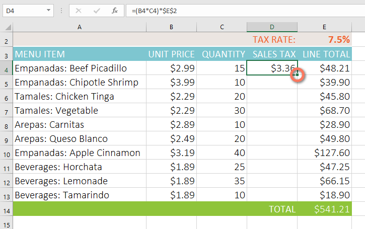
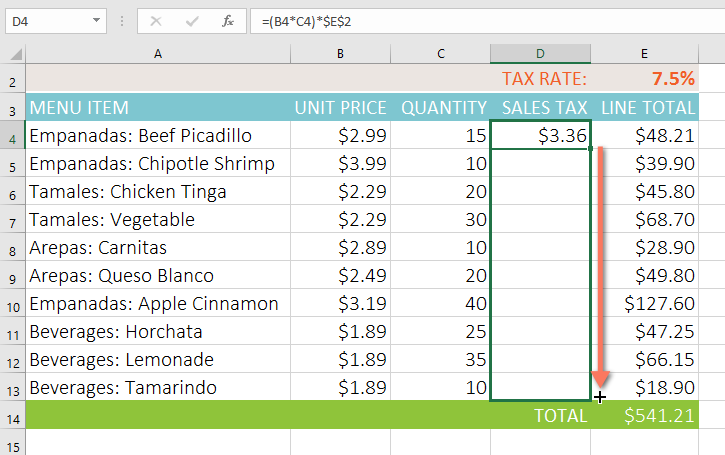
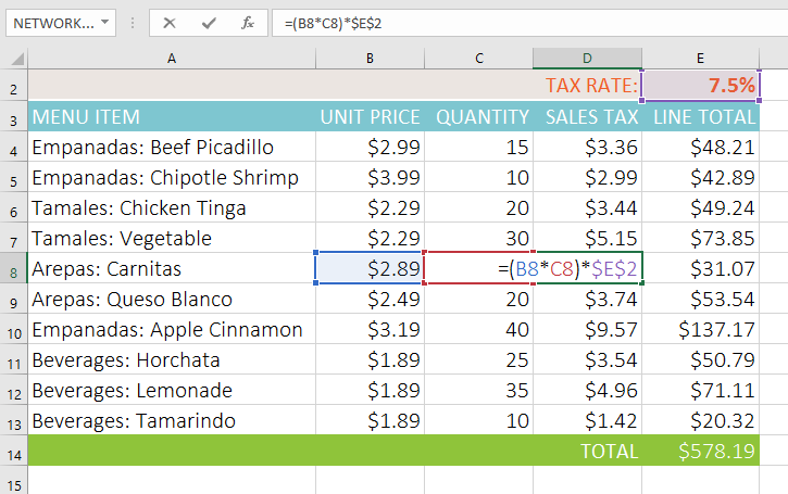
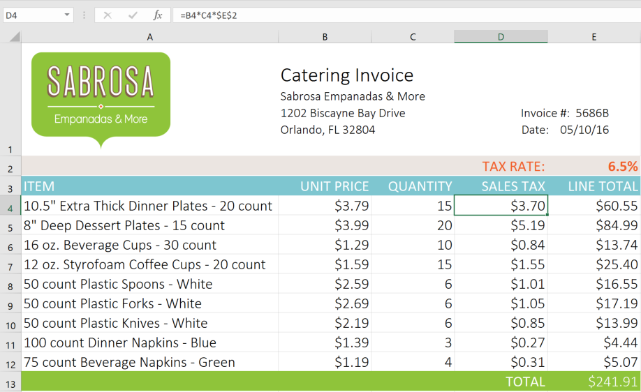
Final Result with Absolute Reference Applied
After locking the tax rate and copying the formula down, every row calculates correctly.
The tax rate remains fixed while unit prices and quantities adjust normally.
Mixed References
Excel allows partial locking of either rows or columns. This is called a mixed reference.
Mixed references are commonly used when building structured financial models or multiplication tables.
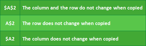
- $A$2 → Fully absolute (row and column locked)
- A$2 → Row locked, column relative
- $A2 → Column locked, row relative
- A2 → Fully relative
Referencing Cells Across Worksheets
You can reference cells from another worksheet using the format SheetName!CellAddress.
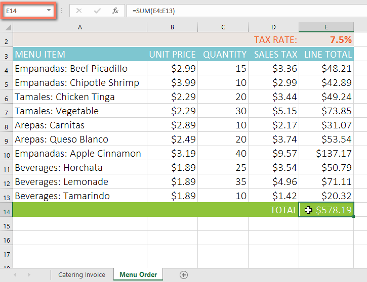
When referencing another worksheet, Excel automatically inserts the sheet name followed by an exclamation point.
If the sheet name contains spaces, Excel will wrap it in single quotation marks. Example: ='Paper Goods'!E13
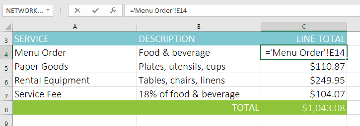
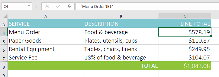
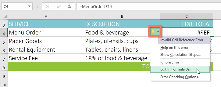
If the sheet name or cell reference is incorrect, Excel will return a #REF! error.
Knowledge Check
Which symbol makes a cell reference absolute in Excel?
Practice File
Download this file and follow along with the lesson.
Challenge
Apply what you've learned in this lesson.
- Download the Cell References practice workbook.
- Click the Paper Goods tab at the bottom-left of the workbook.
Click cell D4 and begin your formula with =.
In cell D4, enter a formula that multiplies the unit price in B4, the quantity in C4, and the tax rate in E2. Make sure to use an absolute reference for the tax rate ($E$2) because it must remain constant.
Use the fill handle to copy the formula to cells D5:D12.
Change the tax rate in cell E2 to 6.5%. If your totals did not update correctly, check whether E2 was locked properly using $E$2.
When you're finished, your workbook should look like this:
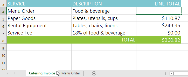
- Click the Catering Invoice tab.
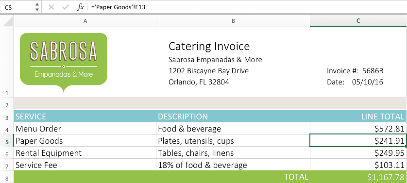
- Delete the value in cell C5 and replace it with a reference to the total cost of the paper goods (cell E13 on the Paper Goods worksheet).
- Use the same steps to calculate the sales tax for each item on the Menu Order worksheet. The total in cell E14 should update.
- In cell C4 of the Catering Invoice worksheet, create a reference to the updated total.
When you're finished, the Catering Invoice worksheet should look like this:
Finished this lesson?
Progress is saved in this browser only. It is not a grade — official progress lives in Brightspace.