Introduction to PivotTables
PivotTables allow you to summarize large datasets instantly and reorganize your data to answer questions quickly.
Video
Watch the lesson video, then complete the reading and challenge.
Lesson Notes
Read through the key concepts before you try the challenge.
Why PivotTables Are Powerful
When a worksheet contains many rows of data, calculating totals manually becomes difficult. PivotTables automatically summarize and analyze large datasets.
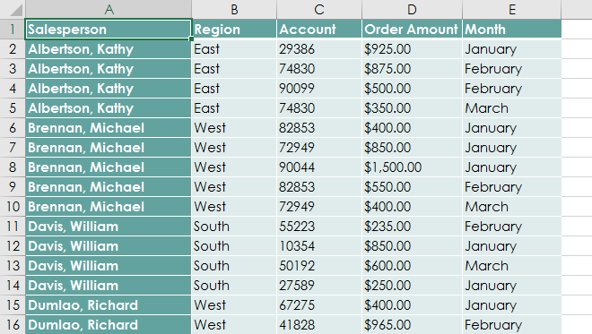
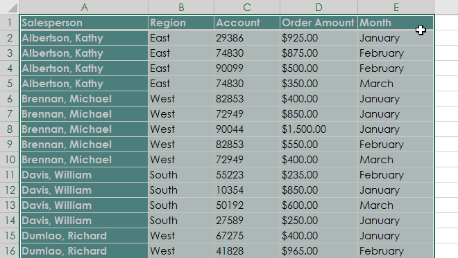
Step 1: Select Your Data
Select the entire dataset including the column headers. These headers will become the fields used in the PivotTable.
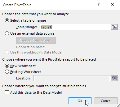
Step 2: Insert the PivotTable
Go to the Insert tab and click PivotTable.
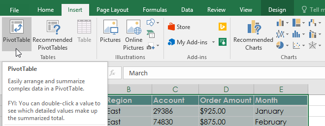
Excel will open the Create PivotTable dialog box.
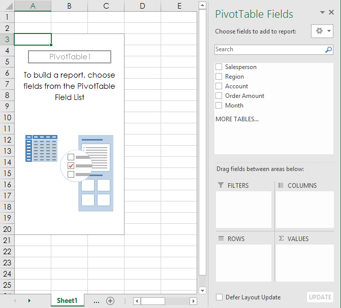
Step 3: Understanding the PivotTable Fields Panel
A blank PivotTable and the PivotTable Fields panel will appear in a new worksheet.
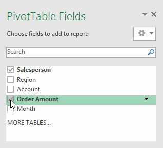
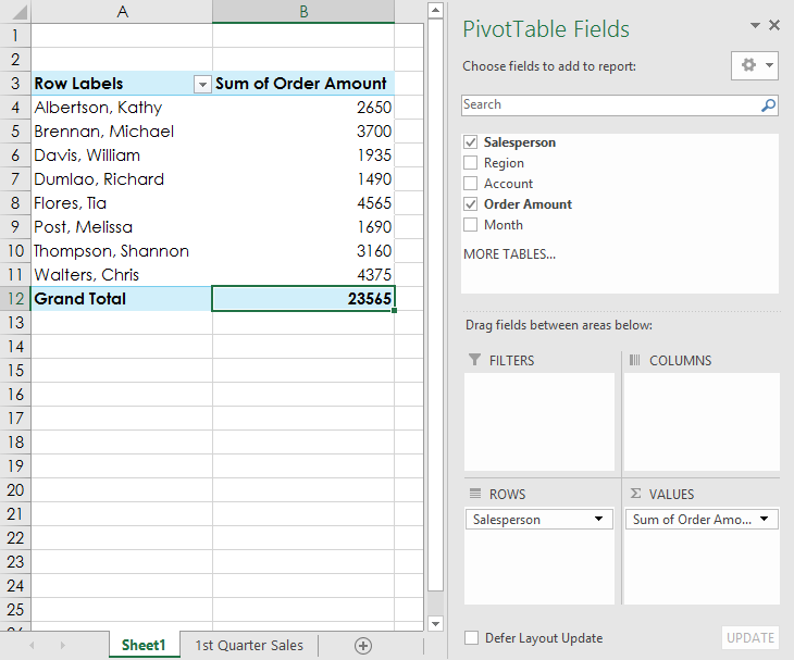
Step 4: Add Fields to Build the PivotTable
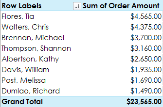
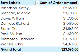
To calculate total sales by salesperson:
- Add Salesperson to the Rows area
- Add Order Amount to the Values area
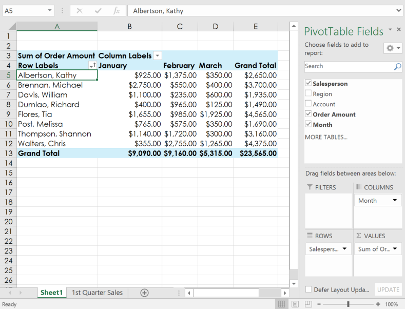
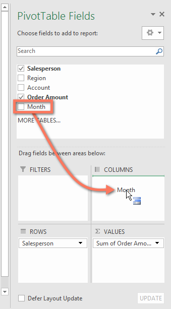
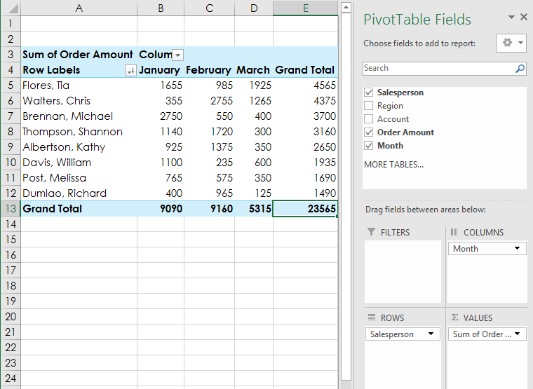
Adding Columns to Analyze More Data
You can analyze the data further by dragging the Month field into the Columns area.
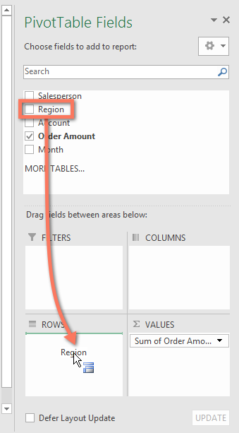
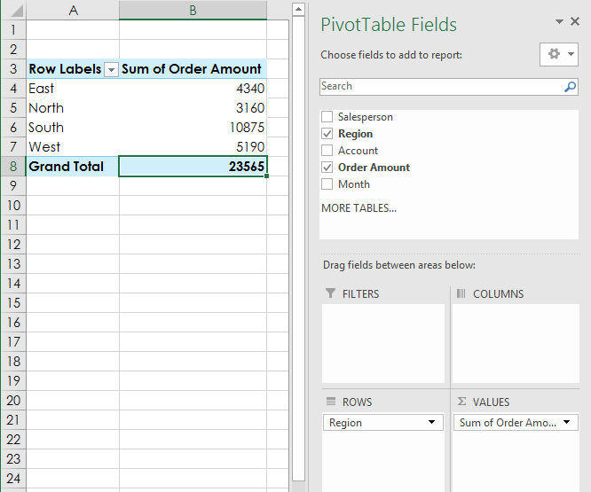
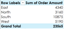
Changing the PivotTable Perspective
PivotTables allow you to reorganize (pivot) the data to answer different questions.
For example, remove Salesperson and instead add Region to see total sales by region.
Sorting and Filtering
PivotTables allow sorting and filtering so you can analyze your data more easily.
Final PivotTable Example
Knowledge Check
What does a PivotTable allow you to do?
Practice File
Download this file and follow along with the lesson.
Challenge
Apply what you've learned in this lesson.
- Open our practice workbook.
- Create a PivotTable in a separate sheet.
- We want to answer the question What is the total amount sold in each region? To do this, select Region and Order Amount.
- In the Rows area, remove Region and replace it with Salesperson.
- Add Month to the Columns area.
- Change the number format of cells B5:E13 to Currency. Note: You might have to make columns C and D wider to see the values.
When you're finished, your workbook should look like this: