Conditional Formatting
Automatically highlight patterns, trends, and performance using Conditional Formatting rules, color scales, data bars, and icon sets.
Video
Watch the lesson video, then complete the reading and challenge.
Lesson Notes
Read through the key concepts before you try the challenge.
Why Conditional Formatting Matters
When working with large datasets, it can be difficult to identify trends and performance issues just by reading numbers. Conditional Formatting automatically applies visual styling based on cell values so patterns become instantly visible.
Step 1: Select the Desired Cells
Before applying Conditional Formatting, select the range of cells you want to evaluate.
Highlight Cells Greater Than a Value
To highlight values greater than a specific number, use the Highlight Cells Rules option.
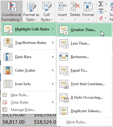
Enter the comparison value (e.g., 4000) and choose a preset style such as Green Fill with Dark Green Text.
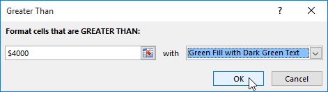
Values above the threshold are automatically highlighted.
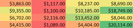
Using Color Scales
Color Scales apply a gradient based on cell values. Highest values receive one color, lowest receive another, and middle values are blended between them.
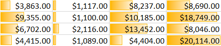
Using Data Bars
Data Bars visually represent values inside each cell using horizontal bars, similar to a mini bar chart.
Using Icon Sets
Icon Sets add symbols such as arrows, circles, or indicators based on value ranges. These are useful for performance dashboards.
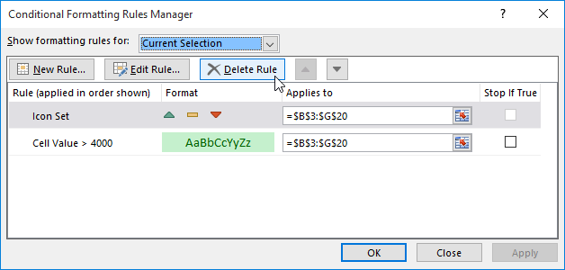
Managing and Editing Rules
Use Manage Rules to edit, delete, or prioritize formatting rules applied to a worksheet.
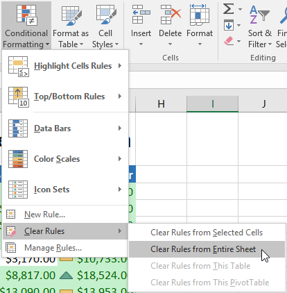
Clearing Conditional Formatting
To remove formatting, click Conditional Formatting → Clear Rules, then choose whether to clear from selected cells or the entire sheet.
Knowledge Check
Which Conditional Formatting option fills cells with a color gradient based on their value?
Practice File
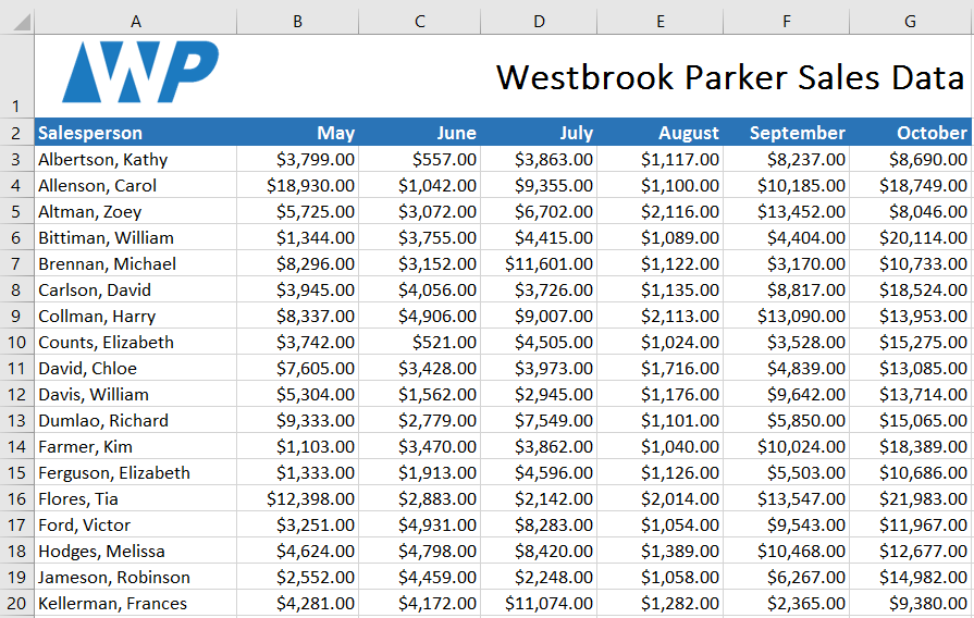
Download this file and follow along with the lesson.
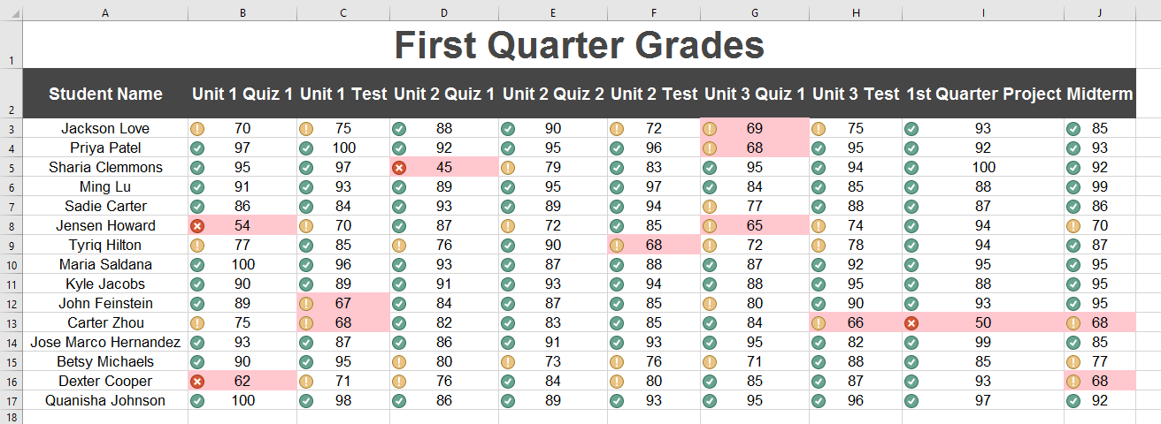
Challenge
Apply what you've learned in this lesson.
Download and open the practice workbook. Then complete the following:
- Click the Challenge worksheet tab.
- Select cells B3:J17.
- Apply Conditional Formatting to highlight values Less Than 70 using a light red fill.
- Apply the Icon Set called 3 Symbols (Circled).
- Use Manage Rules to remove the light red fill rule but keep the icon set.
- Your worksheet should match the example shown below.